Introduction to the Neural Jump ODE framework
In the following we give a brief overview of the considered prediction problem and the Neural Jump Ordinary Differential Equations (NJ-ODEs) framework.
After some presentation videos, we start with an illustrative example to motivate the problem setting and the need for the NJ-ODE framework and then continue with a formal description of the problem setting and the proposed model.
Afterwards, we give short overviews of the different papers about Neural Jump ODEs, outlining their most important contributions.
Finally, we provide a short overview how to get started with the code, if you want to apply NJ-ODEs to your own data.
The videos below are presentations of the papers or parts of them, where the first one is a short general introduction to the framework and the second one
gives more in-depth explanations, focusing on the third paper.
The third video is my PhD presentation, which presents the first five papers in a bit more detail.
In the fourth video, Neural Jump ODE's Forecasting Capabilities in Limit Order Books (LOBs) are discussed, which is covered in the second paper.
Illustrative Example
Vital parameters of patients in a hospital are measured multiple times during their stay. For each patient, this happens at different times depending on
the hospital's resources and clinical needs, hence the observation dates are irregular and exhibit some randomness.
Moreover, not all vital parameters are always measured at the same time (e.g., a blood test and body temperature are not necessarily measure simultaneously),
leading to incomplete observations.
We assume to have a dataset with $N$ patients. For example, patient $1$ has $n_1 = 4$ measurements at hours $(t^{(1)}_1, t^{(1)}_2, t^{(1)}_3, t^{(1)}_4)$
where the values $(x^{(1)}_1, x^{(1)}_2, x^{(1)}_3, x^{(1)}_4)$ are measured.
Patient $2$ only has $n_2 = 2$ measurements at hours $(t^{(2)}_1,t_2^{(2)})$ where the values $(x^{(2)}_1,x^{(2)}_2)$ are measured.
Similarly, the $j$-th patient has $n_j$ measurements at times $(t^{(j)}_1, \dotsc, t^{(j)}_{n_j})$ with measured values $(x^{(j)}_1, \dots, x^{(j)}_{n_j})$.
Each $x^{(j)}_i$ is a $d$-dimensional vector (representing all vital parameters of interest) that can have missing values.
Based on this data, we want to forecast the vital parameters of new patients coming to the hospital. In particular, for a new patient with measured values
$(x_1, \dotsc, x_k)$ at times $(t_1, \dotsc, t_k)$, we want to predict what the vital parameter values will likely be at any time $t > t_k$ for any $0 \leq k \leq n$.
Mathematical Description
Problem Setting
In the simplest form, we consider a continuous-time càdlàg stochastic process $X = (X_t)_{t \in [0,T]}$ taking values in $\mathbb{R}^d$
of which we make discrete, irregular and incomplete observations.
In particular, we allow for a random number of $n\in \mathbb{N}$ observations taking place at the random times
$$0=t_0 < t_1 < \dotsb < t_{n} \le T. $$
For clarification, $n$ is a random variable and $t_i$ are sorted stopping times.
This setup is extremely flexible and allows for a possibly unbounded number of observations in the finite time interval $[0,T]$.
To allow for incomplete observations, i.e., missing values in the observations, we define an observation mask as the sequence of random
variables $M = (M_k)_{k \in \mathbb{N}}$ taking values in $\{ 0,1 \}^{d}$. If $M_{k, j}=1$, then the $j$-th coordinate $X_{t_k, j}$
is observed at observation time $t_k$.
We are interested in online predictions of the process $X$ at any time $t \in [0,T]$ given the observations up to time $t$. Therefore, we define
the information that is available at any time $t$ as the $\sigma$-algebra generated by the observations made until time $t$. In particular, this leads
to the filtration of the currently available information $\mathbb{A} := (\mathcal{A}_t)_{t \in [0, T]}$ given by
$$ \mathcal{A}_t := \boldsymbol{\sigma}\left(X_{t_i, j}, t_i, M_{i} \mid i \leq \kappa(t),\, j \in \{1 \leq l \leq d \mid M_{i, l} = 1 \} \right).$$
The $L^2$-optimal Prediction
We are mainly interested in the $L^2$-optimal prediction of the process $X$ at any time $t \in [0,T]$ given the available information $\mathcal{A}_t$.
This optimal prediction is given by the conditional expectation
$$\hat{X}_t = \mathbb{E}\left[ X_t \mid \mathcal{A}_t \right].$$
While this is a well-defined concept, it is often hard to compute in practice due to the high dimensionality of the process $X$ and the complexity of the information $\mathcal{A}_t$.
Additionally, we do not assume to know the underlying dynamics (i.e., distribution) of the process $X$, but only have access to a training dataset with i.i.d. samples following the description above.
Hence, we propose the Neural Jump ODE as a fully data-driven online prediction model to approximate the optimal prediction $\hat{X}_t$.
Model Architecture of Neural Jump ODEs
We propose a neural network based model, consiting of two main components: a recurrent neural network (RNN) and a neural ODE.
To understand the design of the model architecture, we first review what the model should be able to provide for the online prediction task.
Since we want to have a continuous-time prediction, the model needs to generate an output for every time point $t \in [0,T]$. Between any two (discrete) observation points,
the model does not get any additional information except for the time which evolves and should therefore produce a prediction based on the information at the last observation time and
the current time. This is where the neural ODE comes into play; it is used to model the dynamics of the process (or rather of the optimal prediction $\hat{X}$) between the observation times.
On the other hand, the model should be able to incorporate the information of new observations when they become available. Clearly, a purely ODE-based model would not be able to do this,
as it is deterministic once the initial condition (and driving function) is fixed.
This is where the RNN comes into play; it is used to update the internal model state (i.e., the model's latent variable) $H_t$ at observation times $t_i$ based on the new observation $X_{t_i}$.
Since the new observation leads to a jump in the available information, this will in general also lead to a jump in the model's latent variable at the observation time, $\Delta H_{t_i} = H_{t_i} - H_{t_i-}$.
This model output can be compactly written as the solution $Y$ of the following stochastic differential equation (SDE)
\begin{equation}
\begin{split}
H_0 &= \rho_{\theta_2}\left(X_{0}, 0 \right), \\
dH_t &= f_{\theta_1}\left(H_{t-}, X_{\tau(t)},\tau(t), t - \tau(t) \right) dt + \left( \rho_{\theta_2}\left(X_{t}, H_{t-} \right) - H_{t-} \right) du_t, \\
Y_t &= g_{\theta_3}(H_t),
\end{split}
\end{equation}
where $u_t:=\sum_{i=1}^{n} 1_{\left[t_i, \infty\right)}(t), 0 \le t \le T$ is the pure-jump process counting the current number of observations, $\tau(t)$ is the time of the last observation before or at $t$
and $f_{\theta_1}, \rho_{\theta_2}$ and $g_{\theta_3}$ are neural networks with parameters $\theta_1$, $\theta_2$ and $\theta_3$.
Even though the recurrent structure already allows for path-dependent predictions, we can additionally use the truncated
signature transform as input to the networks $f_{\theta_1}$ and $\rho_{\theta_2}$ (not displayed here).
This often helps the model to better capture the path-dependence of $\hat{X}$, since the signature transform carries important path information that can be hard to capture with the RNN alone.
The Training Framework
Under suitable assumption on the underlying process $X$, this model framework can approximate $\hat{X}_t$ arbitrarily well.
However, to find the optimal parameters $\theta_1, \theta_2$ and $\theta_3$ achieving this approximation, we need a suitable loss function.
In our work we prove that optimizing the loss function
\begin{equation}\label{equ-C0:Psi NJODE1}
\Psi(Z) := \mathbb{E}\left[ \frac{1}{n} \sum_{i=1}^n \left( \left\lvert M_i \odot \left( X_{t_i} - Z_{t_i} \right) \right\rvert_2 + \left\lvert M_i \odot \left( X_{t_i} - Z_{t_{i}-} \right) \right\rvert_2 \right)^2 \right],
\end{equation}
yields the optimal parameters, i.e.,
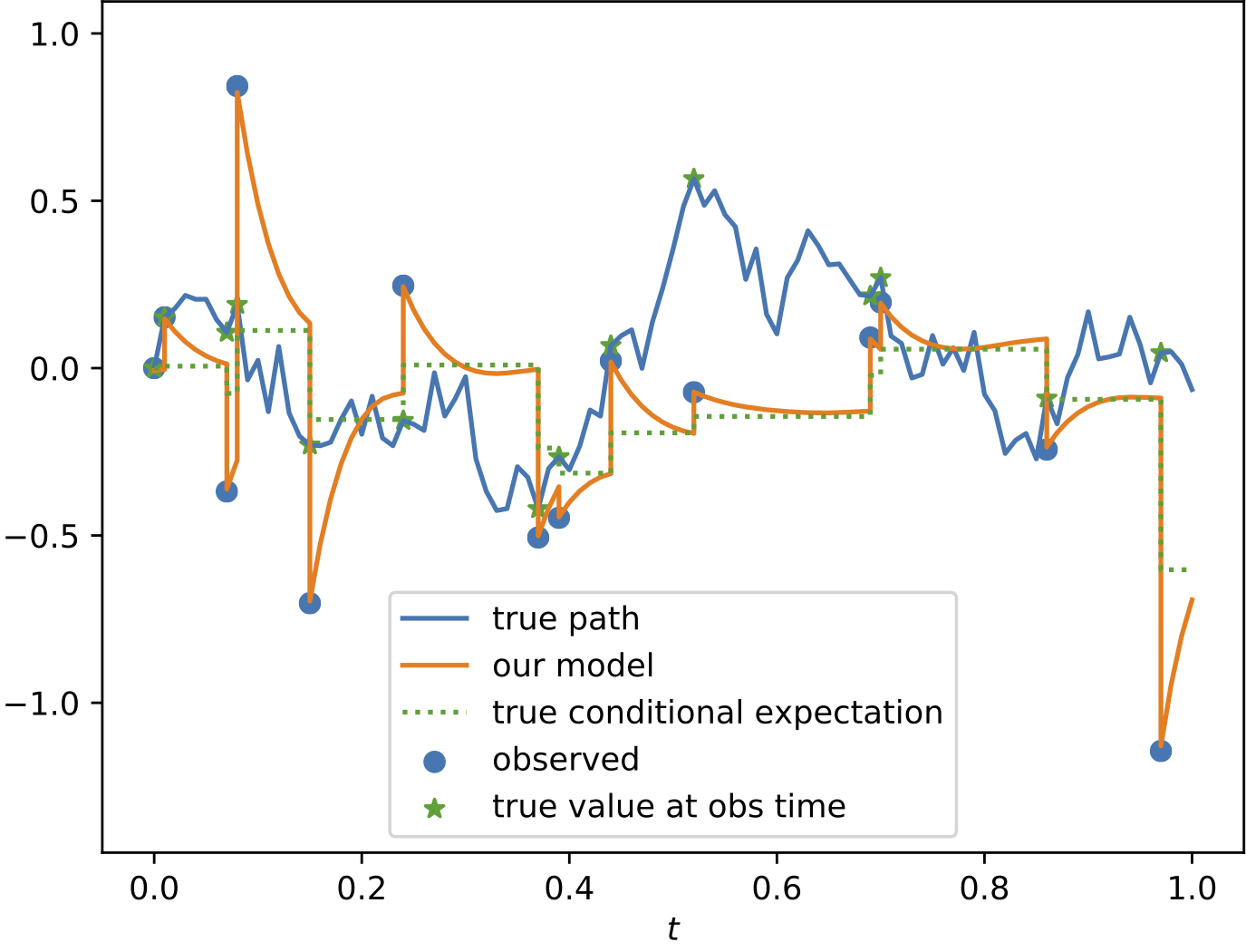
the model output $Y$ converges to the true conditional expectation $\hat{X}$ in the (pseudo) metrics
\begin{equation}\label{equ-C0:pseudo metric}
d_k (Z, \xi) = \mathbb E\left[ \mathbb 1_{\{n \geq k\}} | Z_{t_k-} - \xi_{t_k-} | \right] + \mathbb E\left[ \mathbb 1_{\{n \geq k\}} | Z_{t_k} - \xi_{t_k} | \right],
\end{equation}
for any $k \in \mathbb{N}$.
The intuition for this definition of the loss is that the "jump part" (i.e., the first term) of the loss function forces the RNN
$\rho_{\theta_2}$ to produce good updates based on new observations,
while the "continuous part" (i.e., the second term) of the loss forces the output before the jump to be small in $L^2$-norm.
Since the conditional expectation minimizes the $L^2$-norm, this forces the neural ODE $f_{\theta_1}$ to continuously transform the hidden
state such that the output approximates the conditional expectation well.
Moreover, both parts of the loss force the readout network $g_{\theta_3}$ to reasonably transform the hidden state $H_t$ to the output $Y_t$.
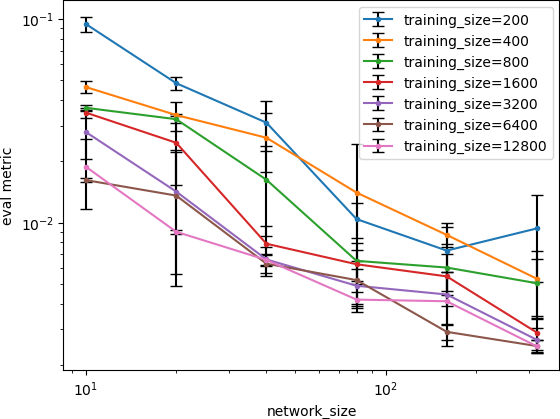
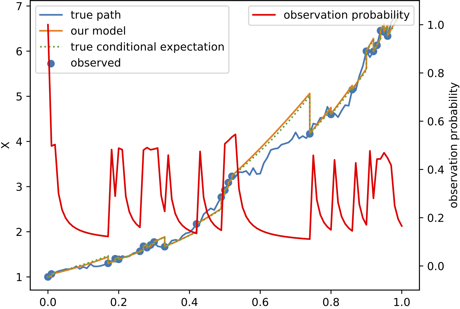
If observations can happen at any time, this intuitively implies that the model has to approximate the conditional expectation well at any time,
since it will otherwise be penalised. Vice versa, if observation never happen within a certain time interval, we cannot guarantee good approximations there,
since then, the training data does not allow for learning the dynamics of the underlying process within this time interval.
Extensions of the Framework
We have extended the basic framework described above in several ways:
- By predicting conditional moments or conditional characteristic functions of $X$, one can use the Neural Jump ODE model to approximate the
conditional law instead of only predicting the conditional mean.
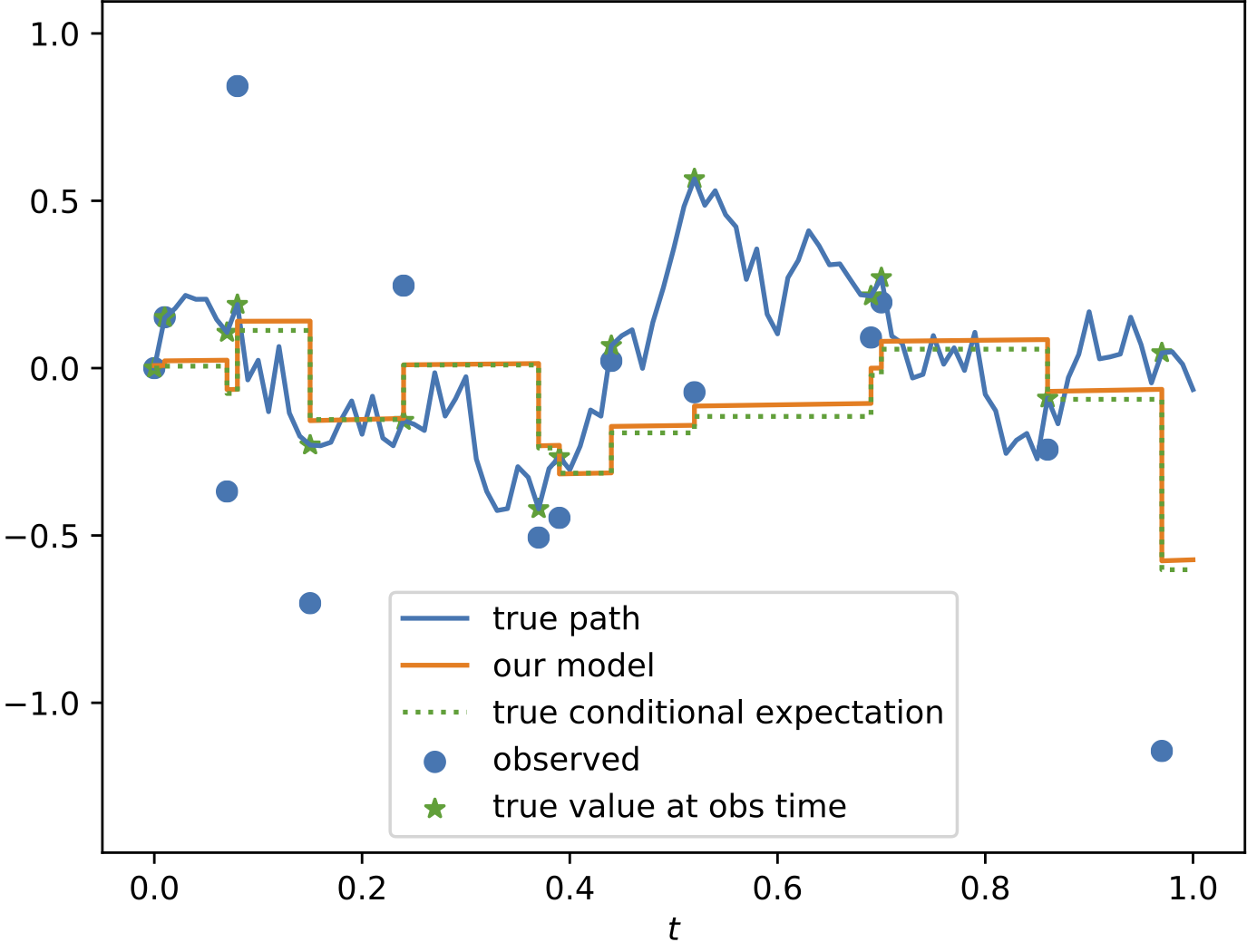
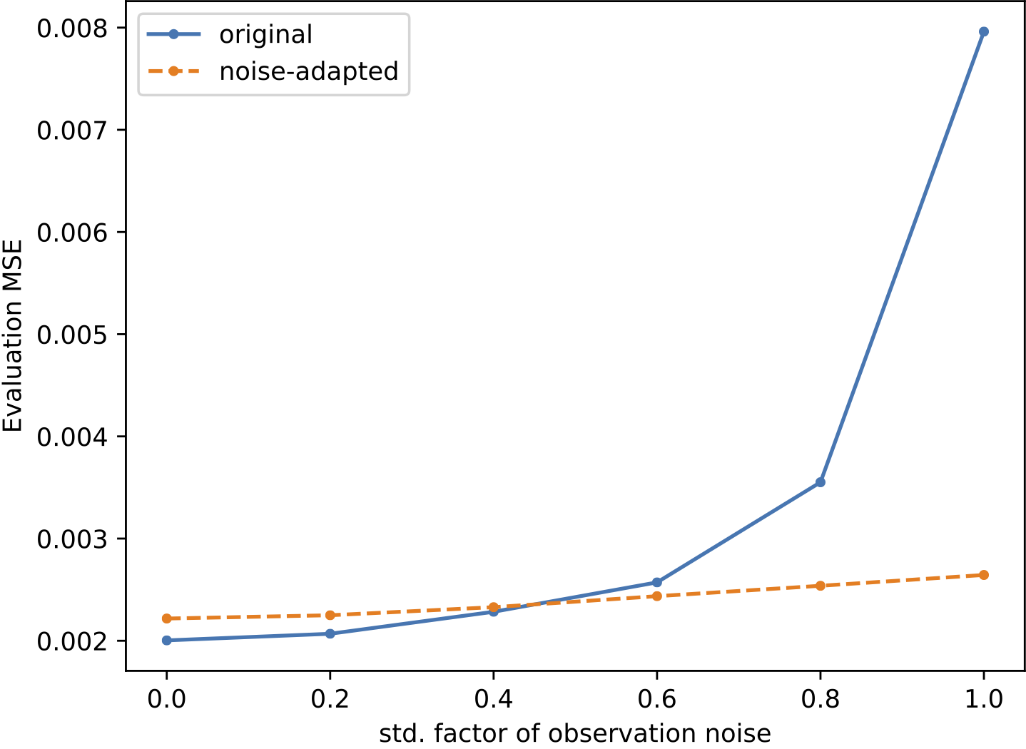
- The noise-adapted loss function can be used if observations of the process $X$ are not noise free.
- Long-term predictions, i.e., approximating $\mathbb{E}\left[ X_t \mid \mathcal{A}_s \right]$ for any $0 \leq s \leq t \leq T$ can be achieved by an
appropriate adaption of the training framework.
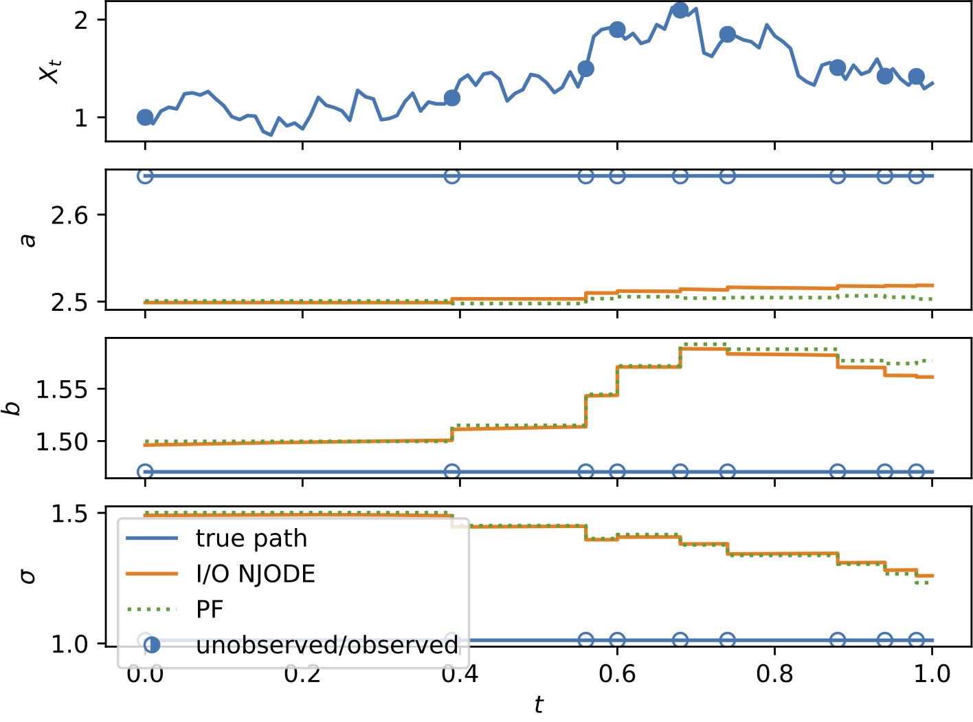
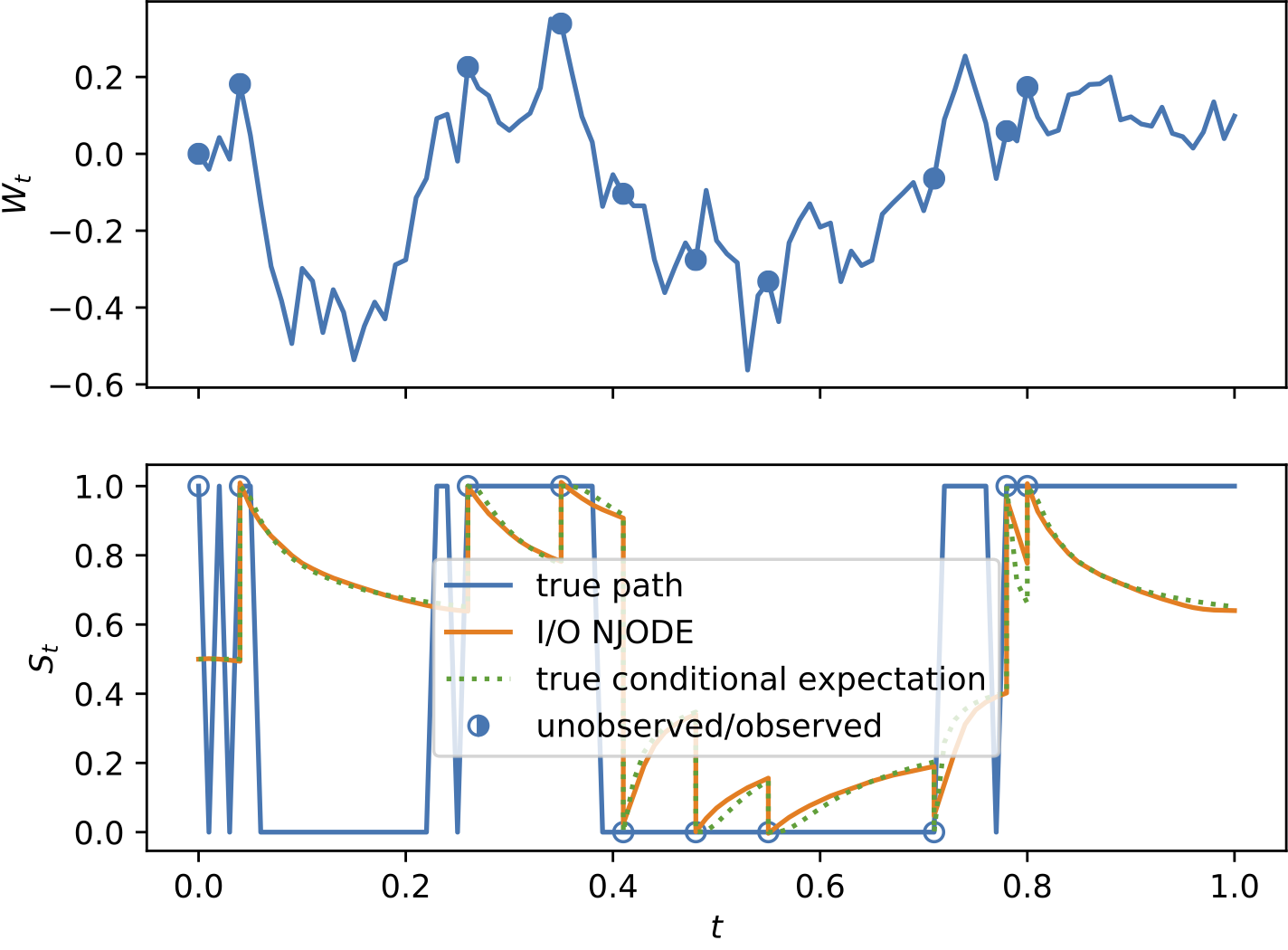
- With the Input-Output loss function the Neural Jump ODE can learn the dynamics of input-output systems, where an output process is
predicted based on observations of an input process. This allows to apply the model for filtering and classification tasks.
- Predicting the conditional mean and variance, the NJODE framework can be used for anomaly detection in time series.
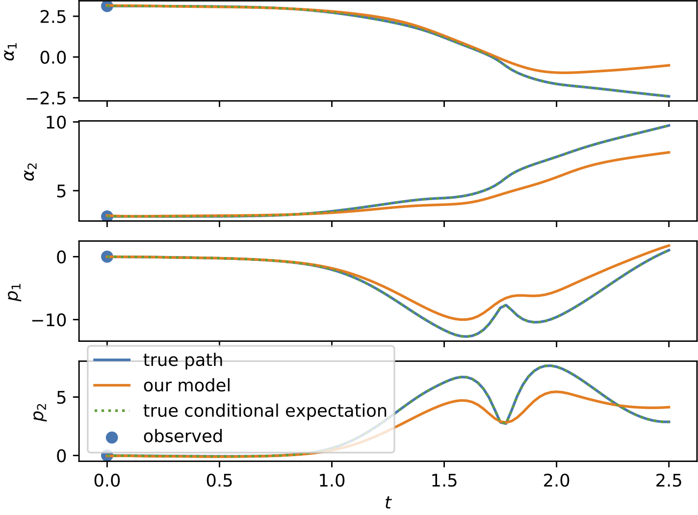
- With new loss functions, the instantaneous coefficients of Ito processes can be learnt with NJODEs and these estimates can be used to generate new paths of the given Ito process.
For more details check out the different
papers.
Considerations Extending Beyond the Paper's Results
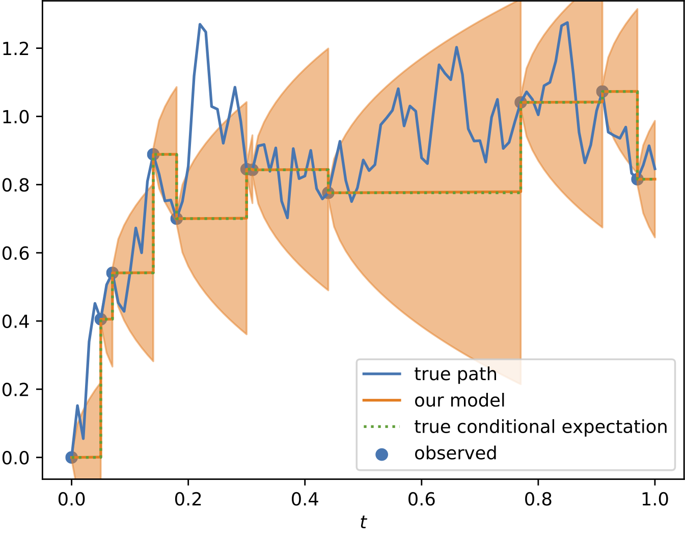
Direct Variance Prediction with the Neural Jump ODE model
Predicting the variance via the first 2 moments can lead to numerical instabilities and therefore implausible negative values or non positive-semi definite covariance matrices.
Instead, we can also directly predict the marginal variance or the covariance matrix using the NJODE model.
In particular, we define the model with two output parts $(Y,W)$, where $Y$ is the original output and $W$ is the variance (of size $d$) or covariance (of size $d^2$) output.
Then we can train $Y$ with the standard loss function to approximate the process $X$, which learns (in the limit) to replicate the conditional expectation $Y_t = \mathbb{E}[X_t | \mathcal{A}_t]$.
Moreover, we train $V=W^2$ (in the marginal variance case) or $V=W^\top W$ (after reshaping, in the covariance matrix case) to approximate the process $(X-Y)^2$.
By using the square $V$ of $W$ to approximate $(X-Y)^2$, we have a hard-coded way to avoid numerical instabilities (negative values of the variance or non positive-semi definite covariance matrices),
since the network output $W$ corresponds to the standard deviation, which is squared to get the variance (in particular, $W$ can have negative entries, which are can be interpreted as being positive).
By the theoretical results, the model output $W$ or $V$, respectively, learns to approximate the conditional expectation of $(X-Y)^2$ arbitrarily well, which coincides with the conditional variance of $X$,
i.e., in the limit we have
\begin{equation}\label{equ:conditional variance}
V_t = \mathbb{E}[(X_t-Y_t)^2 | \mathcal{A}_t] = \mathbb{E}[(X_t- \mathbb{E}[X_t | \mathcal{A}_t] )^2 | \mathcal{A}_t] = \mathbb{E}[X_t^2 | \mathcal{A}_t] - \mathbb{E}[X_t | \mathcal{A}_t]^2 = \text{Var}[X_t | \mathcal{A}_t].
\end{equation}
To be precise, with the definition of the loss function (this is similar to above, except for the $t_i-$ in the second term, which yields the same results for $X$, since $X_{t_i-} = X_{t_i}$ by assumption)
\begin{equation}\label{equ-C0:Psi NJODE1 2}
\Psi(\xi, \zeta) := \mathbb{E}\left[ \frac{1}{n} \sum_{i=1}^n \left( \left\lvert M_i \odot \left( \xi_{t_i} - \zeta_{t_i} \right) \right\rvert_2 + \left\lvert M_i \odot \left( \xi_{t_i-} - \zeta_{t_{i}-} \right) \right\rvert_2 \right)^2 \right],
\end{equation}
we use the loss $\Psi(X,Y)$ to train $Y$ and the loss $ \Psi(Z,V)$ to train $W$, where $Z_t = (X_t - Y_t)^2$, $V=W^2$ (in the marginal variance case) or
$Z_t = (X_t - Y_t)^\top (X_t - Y_t)$, $V=W^\top W$ (in the covariance matrix case), respectively. In the loss function $\Psi(Z,V)$, the $Y$-term in $Z$ is detached from the gradient,
so that the variance loss will only optimize the $W$-term but not the $Y$-term.
We note that $Z_{t-} = (X_{t-} - Y_{t-})^2$ (in the marginal variance case and similar in the covariance matrix case) is in general different from $Z_{t} = (X_{t} - Y_{t})^2$,
since they can differ through $Y$ even if $X_t = X_{t-}$. In particular, $Z_{t_i}=0$ if $X_{t_i} \in \mathcal{A}_{t_i}$ (i.e., fully observed), while $Z_{t_i-}$ is in general not $0$.
Hence, it is important to use $Z_{t_i}$ and $Z_{t_i-}$, respectively, in the 2 terms of the loss function.
One can train 2 models sequentially, first one for $Y$ and then one for $W$, or train 2 independent models jointly, or use the same model with 2 output parts $(Y,W)$.
The latter is the most parameter-efficient, since weight-sharing is used for $Y$ and $W$, which might lead to beneficial transfer learning effects.
However, this might creat a bias through the shared weights, as is always the case when learning more than one output coordinate with the same model.
Jumps at Observation Times
Our assumptions allow for jumps in the process $X$, however, they are not allowed to coincide with observation times.
Nevertheless, this can easily be generalised, if we assume that the process $X$ is observed at the left and the right limit of the observation time, i.e.,
$X_{t_i-}$ and $X_{t_i} = X_{t_i+}$ are observed at the same time $t_i$. Then we can use the loss function $\Psi(\xi, \zeta)$ as defined above
(note that also the process $Z$ for the variance prediction has jumps at the observation times), to recover the same theoretical guarantees.
Explainability in the Context of Neural Jump ODEs
Many ideas of the NJODE framework and extensions are based on explainability arguments.
We created a
jupyter notebook exploring and studying many different aspects of explainability
in the context of NJODEs.
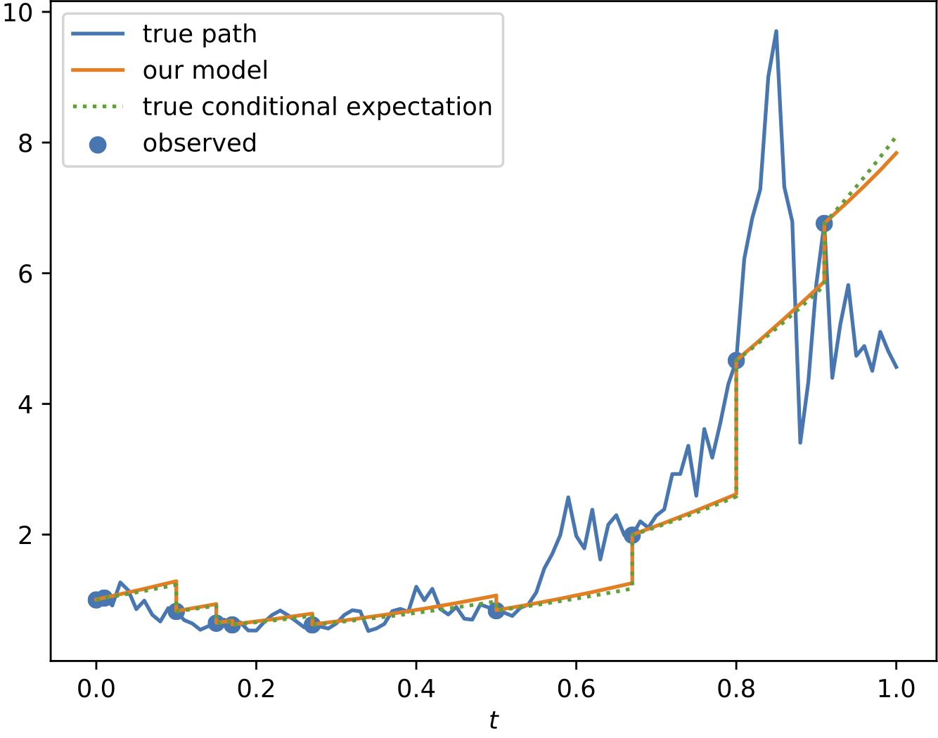
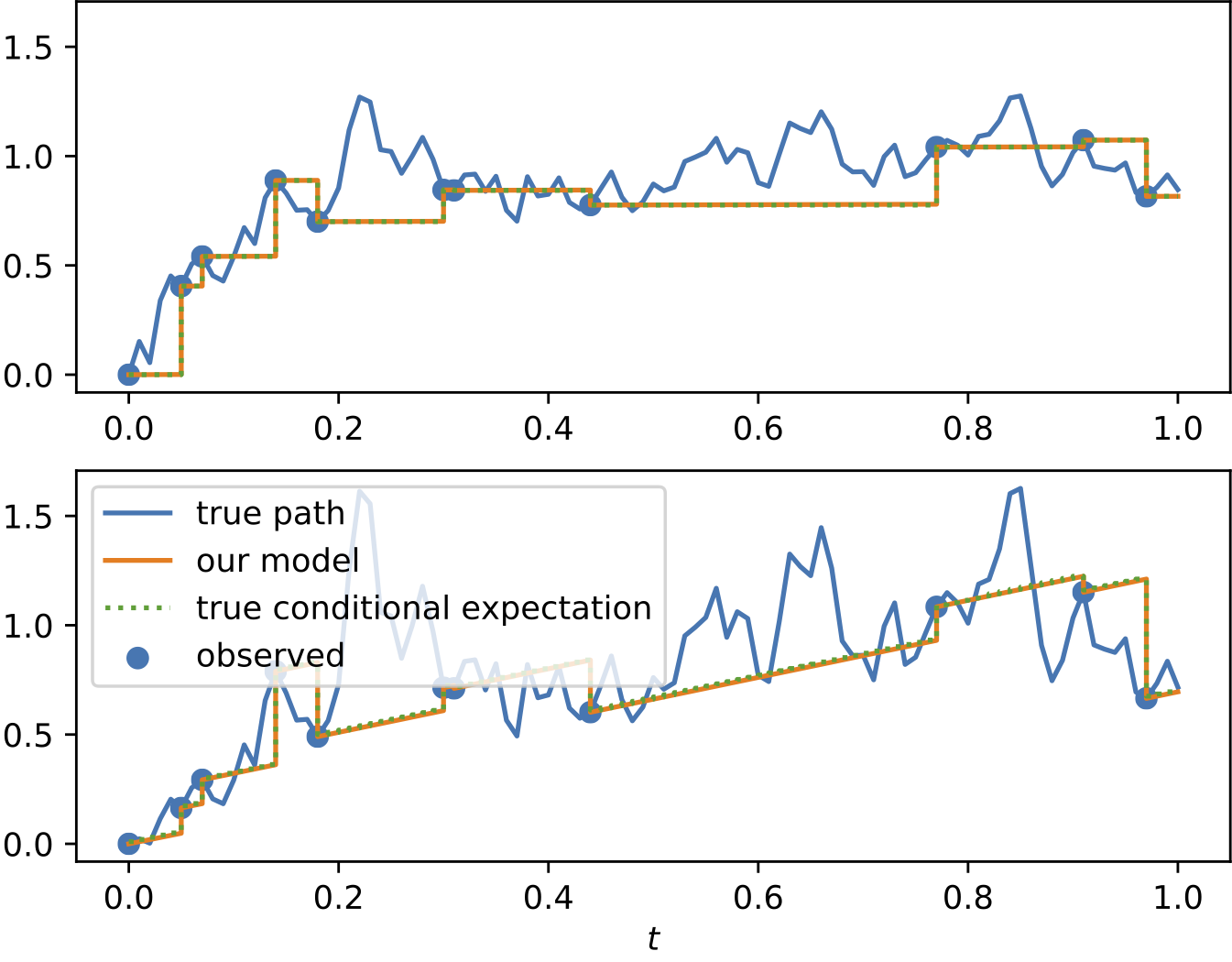
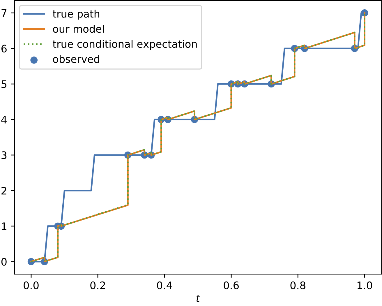
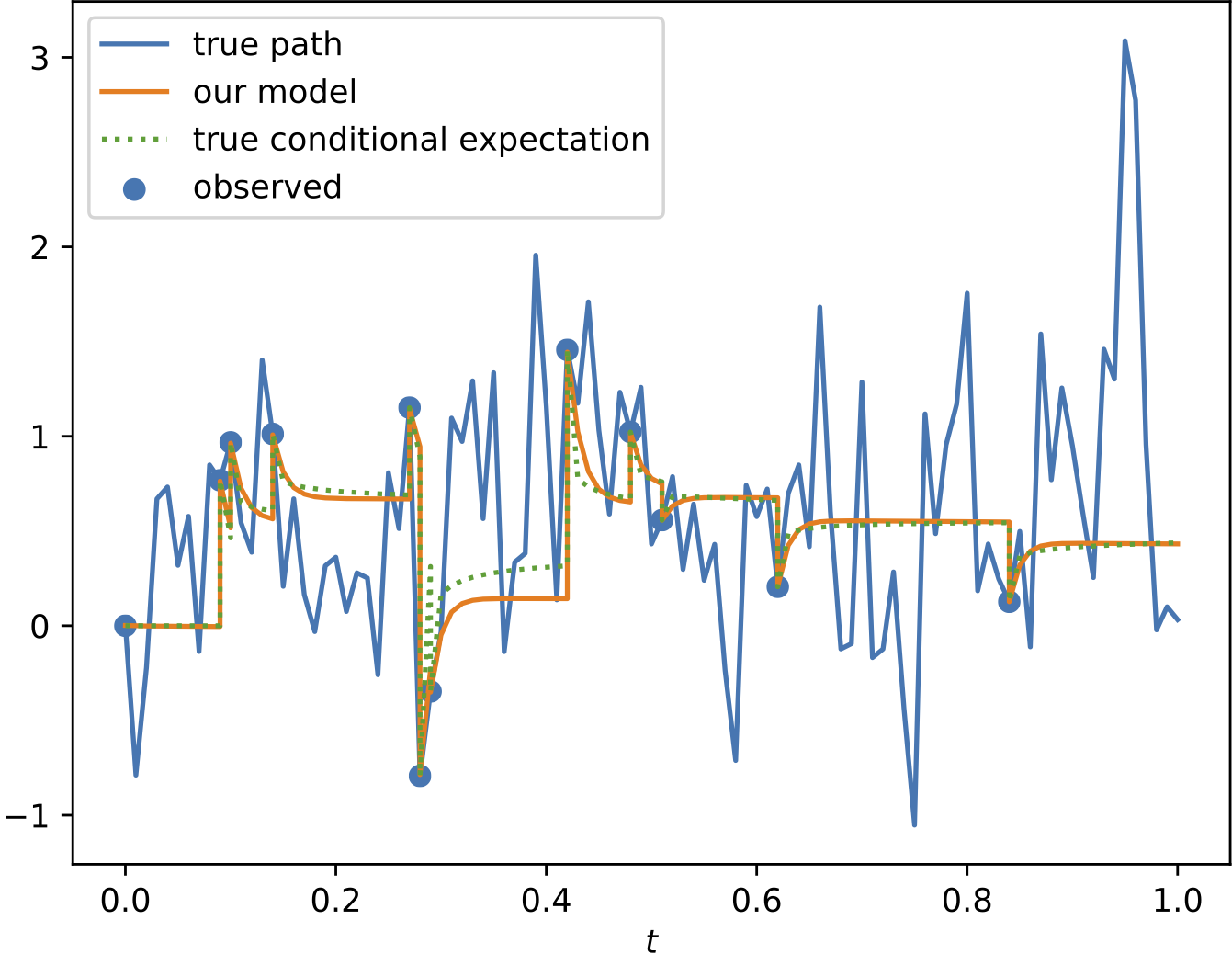
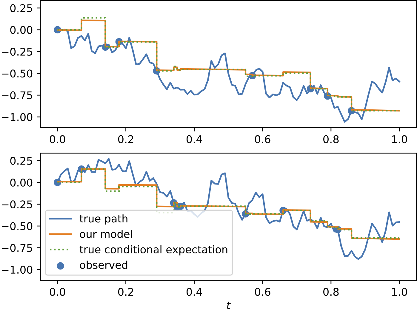
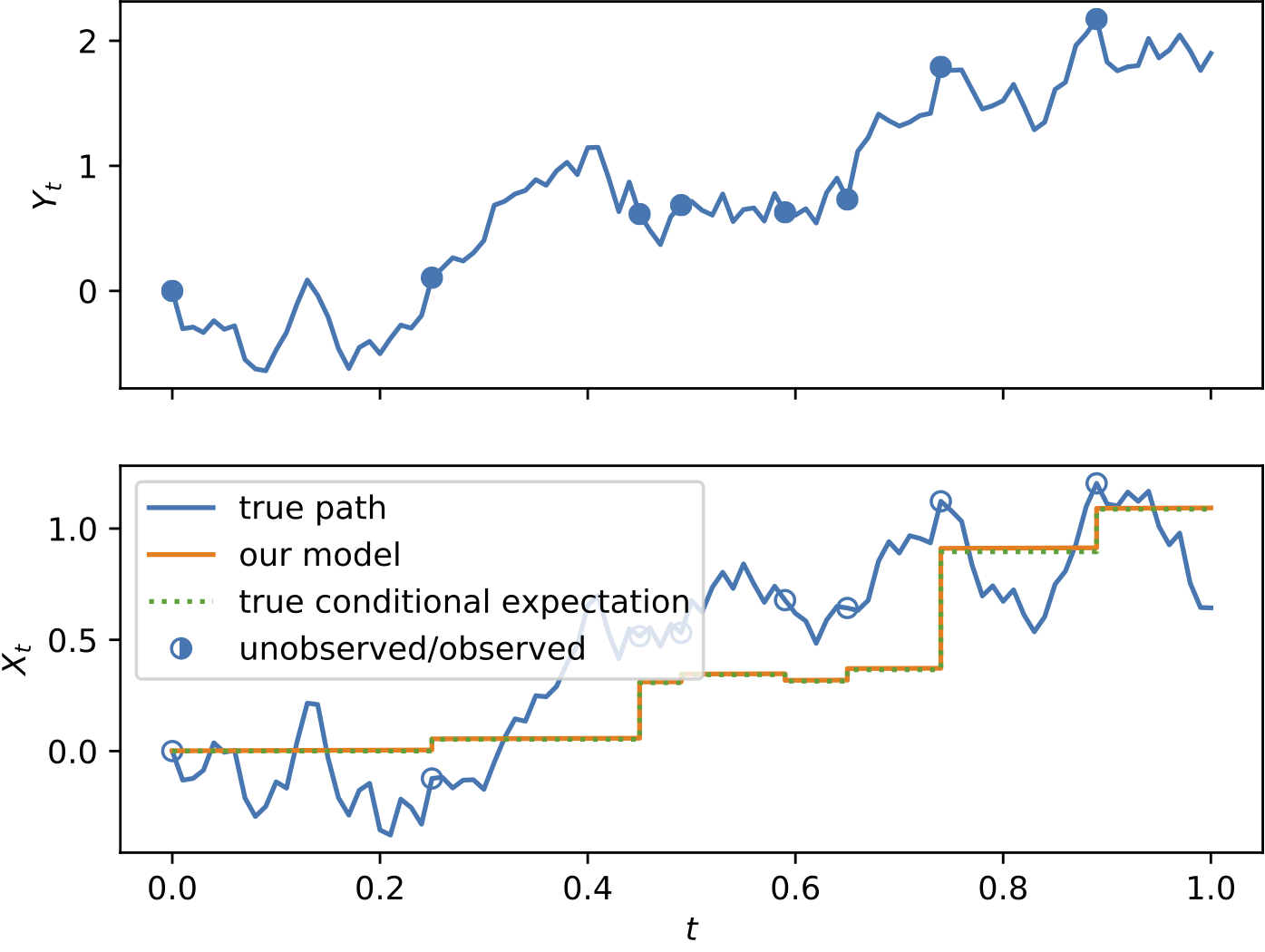
Results
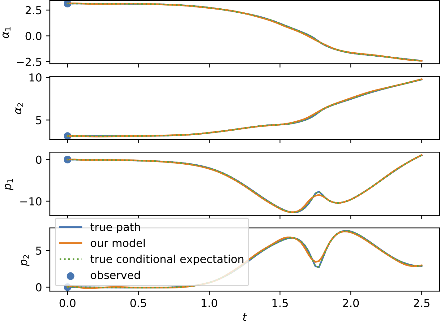
To demonstrate the effectiveness of the proposed model, we provide a series of experiments on synthetic and real-world data.
Some results are shown below. In each of the settings, the model was trained on a training dataset and evaluated on a test dataset,
where also the plots are generated.